Examples#
analitical.follow.py#
import math
import numpy as np
import random
import statistics
import follow
import graph
random.seed(123456)
y = [2, 3]
sigma = 0.1
theta_given_psi = [
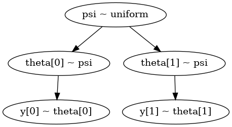
follow.follow("theta[0] ~ psi")(
lambda theta, psi: statistics.NormalDist(psi, 1).pdf(theta[0])),
follow.follow("theta[1] ~ psi")(
lambda theta, psi: statistics.NormalDist(psi, 5).pdf(theta[0])),
]
data_given_theta = [
follow.follow("y[0] ~ theta[0]")(
lambda theta: -(theta[0] - y[0])**2 / sigma**2 / 2),
follow.follow("y[1] ~ theta[1]")(
lambda theta: -(theta[0] - y[1])**2 / sigma**2 / 2),
]
integral = [
graph.Integral(data_given_theta[0],
theta_given_psi[0],
draws=1000,
init=[0],
scale=[0.1],
log=True),
graph.Integral(data_given_theta[1],
theta_given_psi[1],
draws=1000,
init=[0],
scale=[0.1],
log=True),
]
@follow.follow(label="psi ~ uniform")
def likelihood(psi):
return math.prod(fun(psi[0]) for fun in integral)
def prior(psi):
return 1 if -4 <= psi[0] <= 4 else 0
samples = graph.metropolis(lambda psi: likelihood(psi) * prior(psi),
draws=100,
init=[0],
scale=[1.0])
for s in samples:
break
print("has loop:", follow.loop())
with open("analitical.follow.gv", "w") as file:
follow.graphviz(file)
has loop: False
analitical.py#
import math
import matplotlib.pylab as plt
import numpy as np
import random
import statistics
import graph
random.seed(123456)
y = [2, 3]
sigma = 0.1
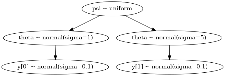
theta_given_psi = [
lambda theta, psi: statistics.NormalDist(psi, 1).pdf(theta[0]),
lambda theta, psi: statistics.NormalDist(psi, 5).pdf(theta[0]),
]
data_given_theta = [
lambda theta: -(theta[0] - y[0])**2 / sigma**2 / 2,
lambda theta: -(theta[0] - y[1])**2 / sigma**2 / 2,
]
integral = [
graph.Integral(data_given_theta[0],
theta_given_psi[0],
draws=1000,
init=[0],
scale=[0.1],
log=True),
graph.Integral(data_given_theta[1],
theta_given_psi[1],
draws=1000,
init=[0],
scale=[0.1],
log=True),
]
def likelihood(psi):
return math.prod(fun(psi[0]) for fun in integral)
def prior(psi):
return 1 if -4 <= psi[0] <= 4 else 0
def fpost(psi):
return 0.4225878520215124 * math.exp(-0.5150415081492156 * psi**2 +
2.100150038994303 * psi -
2.160126048590465)
samples = graph.metropolis(lambda psi: likelihood(psi) * prior(psi),
draws=5000,
init=[0],
scale=[1.0])
psi = np.linspace(-4, 4, 100)
post = [fpost(e) for e in psi]
plt.yticks([])
plt.xlim(-2, 5)
plt.hist([e[0] for e in samples],
50,
density=True,
histtype='step',
linewidth=2)
plt.plot(psi, post)
plt.savefig("analitical.vis.png")
cmaes0.py#
import math
import graph
import matplotlib.pyplot as plt
import random
import sys
import scipy.linalg
def print0(l):
for i in l:
sys.stdout.write("%+7.2e " % i)
sys.stdout.write("\n")
def frandom(x):
return random.uniform(0, 1)
def sphere(x):
return math.fsum(e**2 for e in x)
def flower(x):
a, b, c = 1, 1, 4
return a * math.sqrt(x[0]**2 + x[1]**2) + b * math.sin(
c * math.atan2(x[1], x[0]))
def elli(x):
n = len(x)
return math.fsum(1e6**(i / (n - 1)) * x[i]**2 for i in range(n))
def rosen(x):
alpha = 100
return sum(alpha * (x[:-1]**2 - x[1:])**2 + (1 - x[:-1])**2)
def cigar(x):
return x[0]**2 + 1e6 * math.fsum(e**2 for e in x[1:])
random.seed(1234)
print0(graph.cmaes(elli, (2, 2, 2, 2), 1, 167))
print0(graph.cmaes(sphere, 8 * [1], 1, 100))
print0(graph.cmaes(cigar, 8 * [1], 1, 300))
print0(graph.cmaes(rosen, 8 * [0], 0.5, 439))
print0(graph.cmaes(flower, (1, 1), 1, 200))
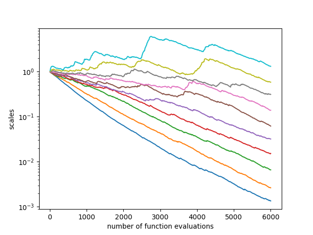
trace = graph.cmaes(elli, 10 * [0.1], 0.1, 600, trace=True)
nfev, fmin, xmin, sigma, C, *rest = zip(*trace)
plt.figure()
plt.yscale("log")
plt.xlabel("number of function evaluations")
plt.ylabel("fmin")
plt.plot(nfev, fmin)
plt.figure()
plt.xlabel("number of function evaluations")
plt.ylabel("object variables")
for x in zip(*xmin):
plt.plot(nfev, x)
plt.figure()
plt.xlabel("number of function evaluations")
plt.ylabel("sigma")
plt.yscale("log")
plt.plot(nfev, sigma)
ratio, scale = [], []
for c in C:
w = [math.sqrt(e) for e in scipy.linalg.eigvalsh(c)]
scale.append(w)
ratio.append(w[-1] / w[0])
plt.figure()
plt.xlabel("number of function evaluations")
plt.ylabel("axis ratio")
plt.yscale("log")
plt.plot(nfev, ratio)
plt.figure()
plt.xlabel("number of function evaluations")
plt.ylabel("scales")
plt.yscale("log")
for s in zip(*scale):
plt.plot(nfev, s)
plt.savefig("cmaes0.png")
-1.80e-01 +2.13e-02 -1.89e-03 +2.55e-04
-1.14e-04 -5.98e-06 +8.51e-05 +8.02e-05 -1.39e-05 +3.30e-05 +6.01e-05 -5.29e-06
+2.97e-04 +4.54e-07 +5.48e-07 -5.03e-07 +1.02e-07 -2.24e-07 +9.78e-08 +5.27e-07
+1.00e+00 +1.00e+00 +1.00e+00 +1.00e+00 +1.00e+00 +1.00e+00 +1.00e+00 +1.00e+00
-5.22e-09 +2.16e-09
coins.py#
import graph
import math
import numpy as np
import pickle
import random
import scipy.stats
import statistics
import sys
random.seed(123456)
n = 250
y = [140, 110]
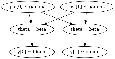
theta_given_psi = [
lambda theta, psi: scipy.stats.beta.pdf(theta[0], a=psi[0], b=psi[1]),
lambda theta, psi: scipy.stats.beta.pdf(theta[0], a=psi[0], b=psi[1]),
]
data_given_theta = [
lambda theta: scipy.stats.binom.pmf(y[0], n, theta[0]),
lambda theta: scipy.stats.binom.pmf(y[1], n, theta[0]),
]
init = [y[0] / n, y[1] / n]
scale = 0.05
draws = 100
integral = [
graph.Integral(data_given_theta[0],
theta_given_psi[0],
draws=draws,
init=[init[0]],
scale=[scale]),
graph.Integral(data_given_theta[1],
theta_given_psi[1],
draws=draws,
init=[init[1]],
scale=[scale]),
]
def prior(psi):
return scipy.stats.gamma.pdf(psi[0], 4, scale=2) * scipy.stats.gamma.pdf(
psi[1], 4, scale=2)
def likelihood(psi):
return integral[0](psi) * integral[1](psi)
samples = graph.metropolis(lambda psi: likelihood(psi) * prior(psi),
draws=50000,
init=[0.1, 0.1],
scale=[1.5, 1.5])
with open("coins.samples.pkl", "wb") as f:
pickle.dump(list(samples), f)
'''
https://allendowney.github.io/BayesianInferencePyMC/04_hierarchical.html#going-hierarchical
'''
coins.vis.py#
import pickle
import numpy as np
import scipy.integrate
import matplotlib.pylab as plt
import statistics
with open("coins.samples.pkl", "rb") as f:
    samples = pickle.load(f)
print(statistics.fmean(e[0] for e in samples))
print(statistics.fmean(e[1] for e in samples))
plt.ylim((0, 0.15))
plt.yticks([])
plt.hist([e[0] for e in samples],
         100,
         density=True,
         histtype='step',
         linewidth=2)
plt.hist([e[1] for e in samples],
         100,
         density=True,
         histtype='step',
         linewidth=2)
plt.savefig("coins.post.png")
8.476043542775162
8.434431620632731
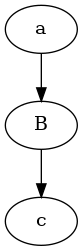
follow0.py#
import follow


@follow.follow()
def a():
    b()


@follow.follow(label="B")
def b():
    c(0)


c = follow.follow(label="c")(lambda i: i, )
a()

print("has loop:", follow.loop())
with open("follow0.gv", "w") as file:
    follow.graphviz(file)
has loop: False
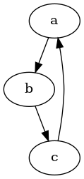
follow1.py#
import follow


@follow.follow()
def a(i):
    if i > 0:
        b(i - 1)


@follow.follow()
def b(i):
    c(i)


@follow.follow()
def c(i):
    a(i)


a(3)

print("has loop:", follow.loop())
with open("follow1.gv", "w") as file:
    follow.graphviz(file)
has loop: True
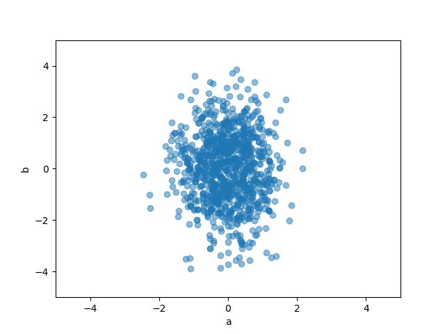
korali0.py#
import graph
import matplotlib.pylab as plt


def fun(x):
    a, b = x
    return -a**2 - (b / 2)**2


samples, S = graph.korali(fun, 1000, [-5, -4], [5, 4], return_evidence=True)
print("log evidence: ", S)
plt.plot(*zip(*samples), 'o', alpha=0.5)
plt.xlim(-5, 5)
plt.ylim(-5, 5)
plt.xlabel("a")
plt.ylabel("b")
plt.savefig("korali0.png")
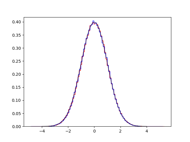
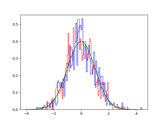
langevin0.py#
import math
import random
import matplotlib.pylab as plt
import graph
import numpy as np


def fun(x):
    return math.exp(-x[0]**2 / 2)


def dfun(x):
    return [-x[0]]


random.seed(123456)
log = False
draws = 1000000
sigma = math.sqrt(3)
step = [1.5]
S0 = graph.langevin(fun, draws, [0], dfun, sigma, log=log)
S1 = graph.metropolis(fun, draws, [0], step, log=log)
x = np.linspace(-4, 4, 100)
y = [fun([x]) / math.sqrt(2 * math.pi) for x in x]
plt.hist([e for (e, ) in S0], 100, histtype='step', density=True, color='red')
plt.hist([e for (e, ) in S1], 100, histtype='step', density=True, color='blue')
plt.plot(x, y, '-k', alpha=0.5)
plt.savefig('langevin0.png')
langevin1.py#
import math
import random
import matplotlib.pylab as plt
import graph
import numpy as np
def fun(x):
return -1 / 2 * (x[0]**2 + x[1]**2)
def dfun(x):
return [-x[0], -x[1]]
random.seed(123456)
draws = 10000
sigma = math.sqrt(3)
S0 = graph.langevin(fun, draws, [0, 0], dfun, sigma, log=True)
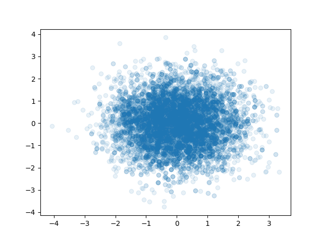
plt.scatter(*zip(*S0), alpha=0.1)
plt.savefig("langevin1.png")
langevin2.py#
import graph
import math
import matplotlib.pyplot as plt
import numpy as np
import tensorflow.compat.v2 as tf
import tensorflow_probability as tfp


def lprob(x):
    return target.log_prob(x)


def fun(x):
    return -1 / 2 * x[0]**2


def dfun(x):
    return [-x[0]]


tfd = tfp.distributions
dtype = np.float32
step_size = 0.75
sigma = math.sqrt(2 * step_size)
target = tfd.Normal(loc=dtype(0), scale=dtype(1))
draws = 1000
S0 = tfp.mcmc.sample_chain(num_results=draws,
                           current_state=dtype(1),
                           kernel=tfp.mcmc.MetropolisAdjustedLangevinAlgorithm(
                               lprob, step_size=step_size),
                           trace_fn=None,
                           seed=42)
S1 = graph.langevin(fun, draws, [0], dfun, sigma, log=True)
x = np.linspace(-4, 4, 100)
y = [math.exp(-x**2 / 2) / math.sqrt(2 * math.pi) for x in x]
plt.hist(S0, 100, histtype='step', density=True, color='red')
plt.hist([e for (e, ) in S1], 100, histtype='step', density=True, color='blue')
plt.plot(x, y, '-g')
plt.savefig('langevin2.png')
langevin3.py#
import graph
import math
import matplotlib.pyplot as plt
import numpy as np
import tensorflow.compat.v2 as tf
import tensorflow_probability as tfp
from tensorflow_probability.python.distributions import mvn_tril
from tensorflow_probability.python.mcmc import sample
from tensorflow_probability.python.mcmc import langevin


def target_log_prob(z):
    return target.log_prob(z)


dtype = np.float32
true_mean = dtype([1, 2, 7])
true_cov = dtype([[1, 0.25, 0.25], [0.25, 1, 0.25], [0.25, 0.25, 1]])
num_results = 500
num_chains = 500
chol = np.linalg.cholesky(true_cov)
target = mvn_tril.MultivariateNormalTriL(loc=true_mean, scale_tril=chol)
init_state = [
    np.ones([num_chains, 3], dtype=dtype),
]
states = sample.sample_chain(
    num_results=num_results,
    current_state=init_state,
    kernel=langevin.MetropolisAdjustedLangevinAlgorithm(
        target_log_prob_fn=target_log_prob, step_size=.1),
    num_burnin_steps=200,
    num_steps_between_results=1,
    trace_fn=None,
    seed=123456)
states = tf.concat(states, axis=-1)
sample_mean = tf.reduce_mean(states, axis=[0, 1])
x = (states - sample_mean)[..., tf.newaxis]
sample_cov = tf.reduce_mean(tf.matmul(x, tf.transpose(a=x, perm=[0, 1, 3, 2])),
                            axis=[0, 1])
print(sample_mean.numpy())
print(sample_cov.numpy())
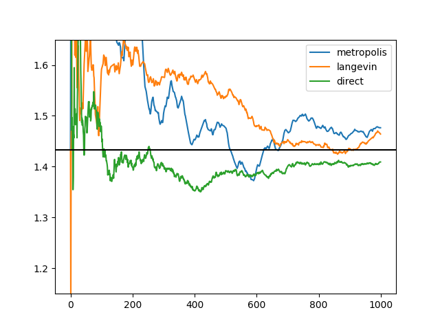
langevin4.py#
import graph
import math
import matplotlib.pylab as plt
import random
import kahan


def fun(x):
    a, b = x
    return -1 / 2 * (a**2 * 5 / 4 + b**2 * 5 / 4 + a * b / 2 - (a + b) * y)


def dfun(x):
    a, b = x
    return (2 * y - b - 5 * a) / 4, (2 * y - 5 * b - a) / 4


def direct(draws):
    for i in range(draws):
        a = random.gauss(y / 3, math.sqrt(5 / 6))
        yield [random.gauss((2 * y - a) / 5, math.sqrt(4 / 5))]


random.seed(123456)
y = 4.3
init = (y / 3, y / 3)
sigma = 1.46
scale = (1, 1)
draws = 1000
for samples, label in ((graph.metropolis(fun, draws, init, scale, log=True),
                        "metropolis"), (graph.langevin(fun,
                                                       draws,
                                                       init,
                                                       dfun,
                                                       sigma,
                                                       log=True), "langevin"),
                       (direct(draws), "direct")):
    mean = kahan.cummean(a for (a, *rest) in samples)
    plt.plot(list(mean), label=label)
    plt.ylim(1.15, 1.65)
plt.axhline(init[0], color='k')
plt.legend()
plt.savefig("langevin4.png")
metropolis0.py#
import graph
import kahan
import scipy.stats
import statistics


def fun(x):
    return scipy.stats.multivariate_normal.logpdf(x, mean, cov)


mean = (1, 2, 7)
cov = ((1, 0.25, 0.25), (0.25, 1, 0.25), (0.25, 0.25, 1))
init = mean
scale = (0.75, 0.75, 0.75)
draws = 40000
S0 = list(graph.metropolis(fun, draws, init, scale, log=True))
x0 = kahan.mean(x for x, y, z in S0)
y0 = kahan.mean(y for x, y, z in S0)
z0 = kahan.mean(z for x, y, z in S0)

xx = kahan.mean((x - x0) * (x - x0) for x, y, z in S0)
xy = kahan.mean((x - x0) * (y - y0) for x, y, z in S0)
xz = kahan.mean((x - x0) * (z - z0) for x, y, z in S0)
yy = kahan.mean((y - y0) * (y - y0) for x, y, z in S0)
yz = kahan.mean((y - y0) * (z - z0) for x, y, z in S0)
zz = kahan.mean((z - z0) * (z - z0) for x, y, z in S0)

print("%.2f %.2f %.2f" % (x0, y0, z0))
print("%.2f %.2f %.2f" % (xx, xy, xz))
print("     %.2f %.2f" % (yy, yz))
print("          %.2f" % zz)
0.97 2.00 6.98
1.03 0.26 0.27
     1.02 0.27
          0.98
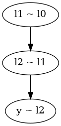
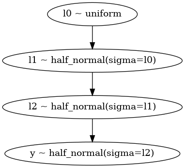
three.follow.py#
import scipy.stats
import graph
import numpy as np
import random
import math
import follow


def prior(psi):
    return 1 if 1 < psi[0] < 40 else 0


seed = 123456
np.random.seed(seed)
random.seed(seed)
data = [0.28, 1.51, 1.14]
l1_given_l0 = follow.follow("l1 ~ l0")(
    lambda theta, psi: scipy.stats.halfnorm.pdf(theta[0], scale=psi[0]))
l2_given_l1 = follow.follow("l2 ~ l1")(
    lambda theta, psi: scipy.stats.halfnorm.pdf(theta[0], scale=psi[0]))
data_given_l2 = follow.follow("y ~ l2")(lambda theta: math.prod(
    scipy.stats.halfnorm.pdf(e, scale=theta[0]) for e in data))
l1 = graph.Integral(data_given_l2,
                    l2_given_l1,
                    draws=10,
                    init=[1],
                    scale=[1.5])
l0 = graph.Integral(l1, l1_given_l0, draws=1000, init=[50], scale=[20])
samples = graph.metropolis(lambda psi: l0(psi) * prior(psi),
                           draws=500,
                           init=[50],
                           scale=[20])
print("has loop:", follow.loop())
with open("three.follow.gv", "w") as file:
    follow.graphviz(file)
has loop: False
three.py#
import scipy.stats
import graph
import numpy as np
import random
import math
import pickle


def prior(psi):
    return 1 if 1 < psi[0] < 40 else 0


seed = 123456
np.random.seed(seed)
random.seed(seed)
data = [0.28, 1.51, 1.14]
l1_given_l0 = lambda theta, psi: scipy.stats.halfnorm.pdf(theta[0],
                                                          scale=psi[0])
l2_given_l1 = lambda theta, psi: scipy.stats.halfnorm.pdf(theta[0],
                                                          scale=psi[0])
data_given_l2 = lambda theta: math.prod(
    scipy.stats.halfnorm.pdf(e, scale=theta[0]) for e in data)
l1 = graph.Integral(data_given_l2,
                    l2_given_l1,
                    draws=1000,
                    init=[1],
                    scale=[1.5])
l0 = graph.Integral(l1, l1_given_l0, draws=1000, init=[50], scale=[20])
samples = graph.metropolis(lambda psi: l0(psi) * prior(psi),
                           draws=50000,
                           init=[50],
                           scale=[20])
with open("samples.pkl", "wb") as f:
    pickle.dump(list(samples), f)
three.vis.py#
import pickle
import numpy as np
import scipy.integrate
import matplotlib.pylab as plt

with open("samples.pkl", "rb") as f:
    samples = pickle.load(f)
D = np.loadtxt("three.dat")
x = D[:, 0]
y0 = D[:, 1]
I0 = scipy.integrate.trapz(y0, x)
plt.yticks([])
plt.hist([e[0] for e in samples],
         40,
         density=True,
         histtype='step',
         linewidth=2)
plt.plot(x, y0 / I0, '-')
plt.savefig("three.vis.png")
tmcmc0.py#
import graph
import math
import random
import scipy.stats
import statistics
import sys


def fun(x, a, b, w, dev):
    coeff = -1 / (2 * dev**2)
    u = coeff * statistics.fsum((e - d)**2 for e, d in zip(x, a))
    v = coeff * statistics.fsum((e - d)**2 for e, d in zip(x, b))
    return scipy.special.logsumexp((u + math.log(w), v + math.log(1 - w)))


sampler = graph.tmcmc
# sampler = graph.korali

random.seed(12345)
D = (
    ("I", 2, 0.5, 0.5),
    ("II", 2, 0.1, 0.9),
    ("III", 4, 0.5, 0.5),
    ("IV", 4, 0.1, 0.9),
    ("V", 6, 0.5, 0.5),
    ("VI", 6, 0.3, 0.5),
    ("VII", 6, 0.1, 0.5),
    ("VIII", 6, 0.1, 0.9),
)
N = 1000
M = 50
beta = 1.0
print("beta = %g" % beta)
for name, d, dev, w in D:
    a = [0.5] * d
    b = [-0.5] * d
    first_peak = []
    smax = []
    logev = []
    for t in range(M):
        x, S = sampler(lambda x: fun(x, a, b, w, dev),
                       N, [-2] * d, [2] * d,
                       beta=beta,
                       return_evidence=True)
        cnt = 0
        for e in x:
            da = statistics.fsum((u - v)**2 for u, v in zip(e, a))
            db = statistics.fsum((u - v)**2 for u, v in zip(e, b))
            if da < db:
                cnt += 1
        first_peak.append(cnt / N)
        smax.append(statistics.fmean(max(e) for e in x))
        logev.append(S)
    cv = lambda a: (statistics.mean(a), 100 * abs(scipy.stats.variation(a)))
    print("%4s %.2f (%.1f%%) %4.2f (%.1f%%) %4.2f (%.1f%%)" %
          (name, *cv(first_peak), *cv(smax), *cv(logev)))
'''
Example 2: Mixture of Two Gaussians
Table 3.Summary of the Analysis Results for Example 2

[0] Ching, J., & Chen, Y. C. (2007). Transitional Markov chain Monte Carlo
method for Bayesian model updating, model class selection, and model
averaging. Journal of engineering mechanics, 133(7), 816-832.

'''
beta = 1
   I 0.50 (4.5%) 0.29 (9.9%) -2.36 (1.7%)
  II 0.90 (2.6%) 0.46 (5.4%) -5.81 (2.5%)
 III 0.48 (7.4%) 0.52 (9.3%) -4.76 (1.9%)
  IV 0.87 (11.0%) 0.48 (20.2%) -11.68 (5.3%)
   V 0.51 (12.0%) 0.66 (10.7%) -7.18 (2.5%)
  VI 0.47 (36.2%) 0.36 (52.1%) -10.63 (5.3%)
 VII 0.55 (54.5%) 0.19 (158.9%) -18.28 (8.6%)
VIII 0.81 (29.4%) 0.45 (53.0%) -18.56 (9.1%)
tmcmc1.py#
import math
import statistics
import graph
import random
import sys


def gauss(x):
    return -statistics.fsum(e**2 for e in x) / 2


random.seed(123456)
sampler = graph.tmcmc
beta = 0.1
N = 2000
M = 50
d = 3
mean = []
var0 = []
var1 = []
var2 = []
lo = -5
hi = 5
for t in range(M):
    x = sampler(gauss, N, d * [lo], d * [hi], beta=beta)
    mean.append(statistics.fmean(e[0] for e in x))
    var0.append(statistics.variance(e[0] for e in x))
    var1.append(statistics.variance(e[1] for e in x))
    var2.append(statistics.variance(e[2] for e in x))
print("%.3f %.4f %.4f %.4f" % (statistics.fmean(mean), statistics.fmean(var0),
                               statistics.fmean(var1), statistics.fmean(var2)))
beta = 0.1
0.011 0.9969 0.9960 1.0063
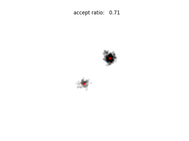
tmcmc2.py#
import graph
import math
import random
import scipy.stats
import statistics
import sys
import matplotlib.pylab as plt


def fun(x, a, b, w, dev):
    coeff = -1 / (2 * dev**2)
    u = coeff * statistics.fsum((e - d)**2 for e, d in zip(x, a))
    v = coeff * statistics.fsum((e - d)**2 for e, d in zip(x, b))
    return scipy.special.logsumexp((u + math.log(w), v + math.log(1 - w)))


random.seed(12345)
beta = float(sys.argv[1])
dev = 0.1
w = 0.9
draws = 500
trace = graph.tmcmc(lambda x: fun(x, [0.5, 0.5], [-0.5, -0.5], 0.9, 0.1),
                    draws, [-2, -2], [2, 2],
                    beta=beta,
                    trace=True)
for i, (x, accept) in enumerate(trace):
    plt.xlim(-2.1, 2.1)
    plt.ylim(-2.1, 2.1)
    plt.gca().set_ymargin(0)
    plt.gca().set_xmargin(0)
    plt.gca().set_axis_off()
    plt.gca().set_aspect('equal')
    plt.subplots_adjust(hspace=0.0, wspace=0.0)
    plt.scatter(*zip(*x), alpha=0.1, edgecolor='none', color='k')
    plt.scatter((0.5, -0.5), (0.5, -0.5), marker='x', color='r')
    plt.title("accept ratio: %6.2f" % (accept / draws))
    plt.savefig("%03d.png" % i)
    plt.close()
smtmcmc.py#
import sys
import statistics
import random
import math
import scipy.special
import numpy as np
import matplotlib.pyplot as plt
import scipy.stats.distributions


def kahan_cumsum(a):
    ans = []
    s = 0.0
    c = 0.0
    for e in a:
        y = e - c
        t = s + y
        c = (t - s) - y
        s = t
        ans.append(s)
    return ans


def kahan_sum(a):
    s = 0.0
    c = 0.0
    for e in a:
        y = e - c
        t = s + y
        c = (t - s) - y
        s = t
    return s


def inside(x):
    for l, h, e in zip(lo, hi, x):
        if e < l or e > h:
            return False
    return True


def fun0(theta, x, y):
    alpha, beta, sigma = theta
    sigma2 = sigma * sigma
    sigma3 = sigma2 * sigma
    M = len(x)
    dif = [y - alpha * x - beta for x, y in zip(x, y)]
    sumsq = statistics.fsum(dif**2 for dif in dif)
    res = -0.5 * M * (math.log(2 * math.pi) +
                      2 * math.log(sigma)) - 0.5 * sumsq / sigma2
    sx = statistics.fsum(x)
    xx = statistics.fsum(x * x for x in x)
    FIM = [[xx, sx, 0], [sx, M, 0], [0, 0, 2 * M]]
    inv_FIM = np.linalg.inv(FIM) * sigma2
    D, V = np.linalg.eig(inv_FIM)
    dd = statistics.fsum(dif)
    dx = statistics.fsum(dif * x for dif, x in zip(dif, x))
    gradient = [dx / sigma2, dd / sigma2, -M / sigma + sumsq / sigma3]
    return res, gradient, inv_FIM, V, D


def fun(theta):
    return fun0(theta, xd, yd)


seed = 123456
np.random.seed(seed)
random.seed(seed)
alpha = 2
beta = -2
sigma = 2
xd = np.linspace(1, 10, 40)
yd = [alpha * xd + beta + random.gauss(0, sigma) for xd in xd]
N = 100
eps = 0.04
d = 3
lo = (-5, -5, 0)
hi = (5, 5, 10)
conf = 0.68
chi = scipy.stats.distributions.chi2.ppf(conf, d)
x = [[random.uniform(l, h) for l, h in zip(lo, hi)] for i in range(N)]
f = [None] * N
out = [None] * N
for i in range(N):
    f[i], *out[i] = fun(x[i])
x2 = [[None] * d for i in range(N)]
f2 = [None] * N
out2 = [None] * N
gen = 1
p = 0
End = False
cov = [[None] * d for i in range(d)]
while True:
    old_p, plo, phi = p, p, 2
    while phi - plo > eps:
        p = (plo + phi) / 2
        temp = [(p - old_p) * f for f in f]
        M1 = scipy.special.logsumexp(temp) - math.log(N)
        M2 = scipy.special.logsumexp(2 * temp) - math.log(N)
        if M2 - 2 * M1 > math.log(2):
            phi = p
        else:
            plo = p
    if p > 1:
        p = 1
        End = True
    dp = p - old_p
    weight = scipy.special.softmax([dp * f for f in f])
    mu = [kahan_sum(w * e[k] for w, e in zip(weight, x)) for k in range(d)]
    x0 = [[a - b for a, b in zip(e, mu)] for e in x]
    for l in range(d):
        for k in range(l, d):
            cov[k][l] = cov[l][k] = beta * beta * kahan_sum(
                w * e[k] * e[l] for w, e in zip(weight, x0))
    ind = random.choices(range(N), cum_weights=kahan_cumsum(weight), k=N)
    ind.sort()
    delta = np.random.multivariate_normal([0] * d, cov=cov, size=N)
    for i, j in enumerate(ind):
        xp = [a + b for a, b in zip(x[j], delta[i])]
        if inside(xp):
            fp, *rest = fun(xp)
            if fp > f[j] or p * fp > p * f[j] + math.log(random.uniform(0, 1)):
                x[j] = xp[:]
                f[j] = fp
        x2[i] = x[j][:]
        f2[i] = f[j]
    if End:
        break
    x2, x, f2, f, out2, out = x, x2, f, f2, out, out2

xmean = [statistics.fmean(x[i] for x in x2) for i in range(d)]
print(xmean)
# print(fun((1.8577, -1.7009, 1.8435), xd, yd))